R进行线性回归和箱线图

# ---------- 安装依赖包（首次运行需执行） ----------
install.packages(c("readxl", "ggplot2", "dplyr", "broom", "ggsci", "scales"))

# ---------- 加载包 ----------
library(readxl)    # 读取Excel
library(ggplot2)   # 绘图
library(dplyr)     # 数据处理
library(broom)     # 统计结果整理
library(ggsci)     # 学术配色
library(scales)    # 科学计数法标签

# ---------- 数据清洗 ----------
# 读取原始数据并处理
df <- read_excel("data.xlsx", sheet = "Sheet1") %>% 
  rename(Year_Season = Year, Birds_Density = `Birds Density`) %>% 
  mutate(
    # 创建时间序号（每半年为一个单位）
    Time_Order = seq(1, nrow(.)),
    # 将年份转换为分类变量（箱线图用）
    Year = substr(Year_Season, 2, 5),  # 直接截取年份部分
    Year = factor(Year),
    Year_Season = gsub("Y", "", Year_Season)  # 美化标签（移除开头的Y）
  )

# ---------- 时间序列回归分析 ----------
# 线性回归（时间序号 vs 鸟类密度）
lm_model <- lm(Birds_Density ~ Time_Order, data = df)

# 提取统计结果
lm_results <- glance(lm_model)
coef_results <- tidy(lm_model)

# 按Nature格式输出结果
cat(sprintf(
  "Time Series Regression:\nSlope = %.1e/year (SE = %.1e)\np = %s\nR² = %.2f",
  coef_results$estimate[2] * 2,  # 转换为年变化率（半年为一个单位）
  coef_results$std.error[2] * 2,
  format.pval(coef_results$p.value[2], digits = 2, eps = 0.001),
  lm_results$r.squared
))

# ---------- 学术级时间序列图 ----------
ggplot(df, aes(x = Time_Order, y = Birds_Density)) +
  geom_point(size = 4, shape = 21, fill = "#4DBBD5FF") +
  geom_smooth(method = "lm", color = "black", formula = y ~ x) +
  scale_x_continuous(
    breaks = df$Time_Order,
    labels = df$Year_Season
  ) +
  scale_y_continuous(labels = scientific_format()) +  # y轴科学计数法
  labs(
    x = "Time Period", 
    y = expression(Birds~Density~(individuals~km^{-2})),
    title = "Temporal Trend of Bird Density"
  ) +
  theme_classic(base_size = 12) +
  theme(
    text = element_text(family = "Arial"),
    axis.text.x = element_text(angle = 45, hjust = 1),
    plot.title = element_text(hjust = 0.5, face = "bold")
  ) -> p_trend

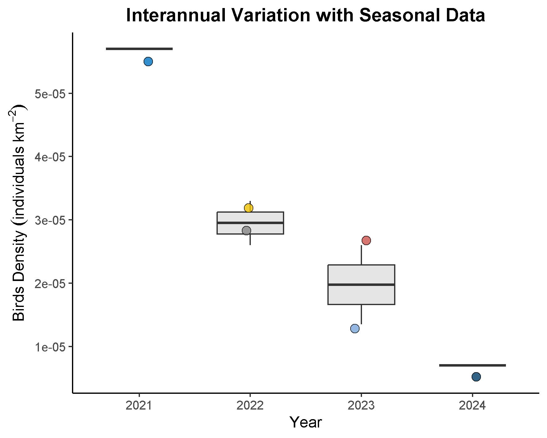
# ---------- 按年份的箱线图（含原始数据点） ----------
ggplot(df, aes(x = Year, y = Birds_Density)) +
  geom_boxplot(width = 0.6, fill = "gray90", outlier.shape = NA) +
  geom_jitter(aes(fill = Year_Season), 
              width = 0.1, size = 3, shape = 21, alpha = 0.8) +
  scale_fill_jco() +  # JAMA期刊配色
  scale_y_continuous(labels = scientific_format()) +
  labs(
    x = "Year", 
    y = expression(Birds~Density~(individuals~km^{-2})),
    title = "Interannual Variation with Seasonal Data"
  ) +
  theme_classic(base_size = 12) +
  theme(
    text = element_text(family = "Arial"),
    legend.position = "none",
    plot.title = element_text(hjust = 0.5, face = "bold")
  ) -> p_box

# ---------- 显示并保存图表 ----------
print(p_trend)
print(p_box)

ggsave("time_trend.jpg", p_trend, 
       width = 18, height = 12, units = "cm", dpi = 300)
ggsave("year_boxplot.jpg", p_box, 
       width = 15, height = 12, units = "cm", dpi = 300)